Estimating ADWF at sewage treatment plants

D de Haas, S Ng, N Dahl, D Baulch.

First published in Water e-Journal Vol 6 No 1 2021.

DOWNLOAD THE PAPER

Abstract

Estimating and understanding Average Dry Weather Flow (ADWF) is fundamental to the planning, design, and operation of sewage treatment plants (STPs). This paper reviewed methods for estimation of ADWF, in four general groups: Rainfall-based; Equivalent person (EP) based; Basic statistical (Percentiles); and ‘Novel’. The ‘Novel’ methods identified were: Histogram/ Mode; Antecedent Precipitation Index (API); Ratio of Short Term and Long-Term Moving Averages; K-means Clustering; Diurnal Profile Smoothing; and Kernel Density Estimation. EP-based methods were not considered useful because they shift the uncertainty from rainfall and/or flow data to population and/or loading data. The other methods were tested using datasets for two STPs of similar size (ADWF approximately 1.2 to 1.3 ML/d) in northern New South Wales, one of which is more prone to wet weather inflow/ infiltration (I/I). On balance of simplicity and performance against more complex methods, we recommend the Histogram/ Mode and/or the Percentile methods for routine reporting. For larger and more complex assignments (e.g., design projects, planning studies), it is recommended that one or more of the alternative high-performing methods described in this paper (e.g., Ratio of moving averages; Kernel Density Estimation) be employed for ADWF checks. Relatively large datasets (at least one year of daily flow totals) should be used and the results compared against the estimates from simpler methods.

Introduction

Historically, both locally and internationally, engineers and managers of water utilities have applied various methods to determine the average dry weather flow (ADWF) for sewage treatment plants (STPs). To our knowledge, at least in Australia, there is no single industry standard method to define or determine ADWF. Common methods (typically) apply some form of numerical ‘filter’ to the totalised daily data for STP inflow, based on concurrent rainfall records. Such methods vary in detail (e.g., number of days, rainfall amount etc. applied to the numerical filter). Furthermore, such methods are constrained by the issue of representative rainfall data to apply for STP catchments (e.g., accuracy of rainfall records, nearest geographic factors, spatial distribution of rainfall) and the variable degree to which rainfall affects STP inflows (e.g., prolonged effects of rainfall on infiltration/ inflow (I/I) in some but not all catchment sewer systems).

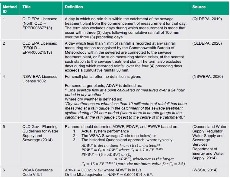
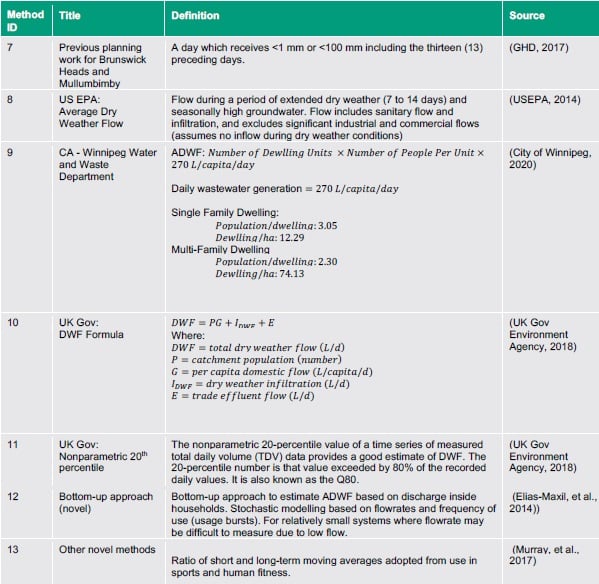
A review of industry ‘best practice’ methods for defining and calculating ADWF at STP was collated from various sources, including the following: existing environmental licenses in Australia (QLD and NSW); international governing bodies (UK Government Environment Agency and Winnipeg Water and Waste Department); and industry practice (e.g., previous approaches used by consultants, suggested alternatives by local councils, or industry associations etc.).

The methods reviewed fell into four groups:

1. Rainfall-based
2. EP based
3. Basic statistical
4. Novel

Rainfall-based methods attempt to determine which days were dry by examining historical daily rainfall records and, in many cases, also looking at rainfall on a given day along with preceding days.

EP-based methods attempt to determine dry weather flow empirically by estimating the number of equivalent persons (EP) within the catchment area and multiplying by an average wastewater production per EP.

Basic statistical methods were those that apply a very simple statistical analysis of flow data. The only example of this found in the literature review was Percentile-based estimations; however, using a histogram or mode calculation would be very similar. Percentile-based methods look at the entire set of flow data, including wet days, and estimate the average dry weather flow by taking a flow percentile (typically between the 20^th and 50^th percentile). The histogram/ mode method looks at the frequency of different flowrates and takes the most commonly occurring flowrate as an estimate for ADWF.

‘Novel’ methods were those that did not fall into one of the other three groups described above. In the literature review, only one method was considered novel, namely a ‘ground-up’ approach for very small flow systems. The average flow for household water-using devices (taps, showers, appliances etc.) is estimated and ADWF is then stochastically estimated based on the frequency and duration of use.

The aim of this paper was to compare the results of using the current industry ‘best practice’ methods for estimating ADWF against five novel estimation methods that seek to improve estimate performance. To our knowledge, the novel methods we selected for testing have never been applied for this purpose to STP flows on a routine basis.

Methodology

Data

Flow data from 2011 to 2020 was supplied by Byron Shire Council (BSC) for two sewage treatment plants (STP) in northern New South Wales: Ocean Shores STP (OSSTP) and Brunswick Valley STP (BVSTP). The two plants are located within a straight-line distance of 1.7 km from each other.

Additional short time interval flow rate data from 2017 to 2019 was provided for BVSTP for use in the Diurnal Profile Smoothing method, as described below.

Rainfall data was retrieved from the nearby weather stations from Bureau of Meteorology (BOM) data: Mullumbimby and Brunswick Heads Bowling Club (BOM station no. 058040 and 058103, respectively).

Overview

Investigations began with a preliminary set of estimates using current industry methods. The initial methods tested were:

• 20^th percentile
• 30^th percentile
• 50^th percentile
• QLD EPA SEQ Rainfall-based method
• One-week Rainfall-based method
• Three-week Rainfall-based method.

These informed the initial rating system for discerning good vs. poor estimates. To do this, the above-mentioned methods were separated into three levels of strictness: Least Strict, Moderately Strict, and Strictest. The Strictest estimates were expected to be the highest performing as they eliminated the most data for days influenced by rainfall events.

Six additional methods were proposed - one basic statistical, and five ‘novel’ methods - as follows:

• Histogram / Mode (basic statistical method)
• Antecedent Precipitation Index (API)
• Ratio of Short Term and Long-Term Moving Averages
• K-means Clustering
• Diurnal Profile Smoothing
• Kernel Density Estimation

Each method was evaluated and compared against the results of the Strictest estimates from the above-mentioned rating of the initial methods tested. Based on the highest performing among the initial and proposed additional methods, a ‘true value ADWF’ was adopted for the datasets examined from each of the two STPs.

To assess the ability of individual methods to estimate ADWF, the results for each were compared against the ‘true value ADWF’ for the two STPs and a relative score given. All methods were then compared in a Multi-Criteria Assessment (MCA), which scored the methods semi-quantitatively for Estimate Performance, Data Requirements, Mathematical Complexity, Parameter Complexity, and Robustness.

Description of novel estimation methods

Antecedent Precipitation Index (API) Method

The first novel method is similar to rainfall-based methods. It applies an established modelling term, namely Antecedent Precipitation Index (API). API is a running day-by-day index of moisture stored within a drainage basin (Ali, et al., 2010). The difference between API versus a simple cumulative rainfall is that API considers the nature of catchments where drying out progressively occurs during periods without rain, making recent rainfall events more impactful than earlier events. Mathematically, API takes the form of:

Where:

i is the number of antecedent (preceding) days considered

k is the decay constant (d^-1)

P_t is the rainfall during a given day at time, t

t is time (days).

For this study, the values we chose for k and i were 0.9
(Ali et al., 2010; Kohler & Linsley, 1951) and 27 days, respectively. This approach considers rainfall over the 27 antecedent days up to and including a given present day (28 days total). The index progressively places less weighting on rainfall that occurred in earlier antecedent days, culminating in a weighting of 5% for rainfall measured on the 27^th antecedent day.

We defined a dry day as any day with. Using this definition, ADWF was then calculated as the median of dry day flows.

Ratio of short term and long-term moving averages

The second novel method is based on the ratio of short-term to long-term moving averages of daily flows. Based on similar applications for monitoring variance within natural systems, including human fitness (Murray et al., 2016), this method compares the short and long-term averages to determine if flow is changing significantly or relatively stable. A ratio between the short and long-term averages close to unity (1.0) is taken as an indicator of stable flow and, by implication, dry weather flow.

This method has the benefit that it technically does not classify “dry weather” based on rainfall but rather attempts to discern baseline flows. This has the advantage that it can be equally applied in regions with different climates, including those where rainfall occurs relatively frequently, causing I/I to produce on-going contributions to average flow. Similarly, it can be applied in situations where local rainfall records either do not exist or are unreliable. By contrast, rainfall-based methods depend on reliable rainfall data and a single definition of ‘dry weather’ is difficult for different situations.

Arithmetic moving average

The simplest form of calculating moving averages is arithmetically. In this case the moving average is the sum of flowrates divided by the number of days considered. Mathematically, the formula is:

Where:

F is the moving average

i is number of days considered

t is the time (days)

F_t is the flowrate on day t

For this study, we chose i to be 7 days (1 week) for the short-term average, and 28 days (4 weeks) for the long-term average. The ratio of short-term average to long-term average (ϕ) is simply expressed as:

Where F_ST and F_LT are the short term and long-term moving averages, respectively.

To classify dry weather days, by trial and error we selected an upper bound for the ratio (ϕ) of 1.025 and a lower bound 0.976 (the inverse of the upper bound).

Exponentially weighted moving average

The exponentially weighted moving average (EWMA) is a modification to the arithmetic moving average where a diminished weighting is applied to older flowrates, like the API method. The formula for the EWMA is:

Where:

F is the moving average

i is the number of days considered

t is time (days)

F_t is the flowrate on day ‘t’

k is the decay constant.

As before, we chose value of i = 7 days for the short-term average, and i = 28 days for the long-term average. We chose k to be 0.9, consistent with the API method (see above). As before, to classify dry days we chose an upper bound for the ratio of 1.025 and a lower bound of 0.976.

Ratio of moving averages with step-change limit

A modification of the Ratio of Moving Averages method was developed to limit the impact on results from large rainfall events. This modification excludes readings where the ratio of averages changes rapidly. For example, after a heavy rainfall event the short-term moving average flow spikes to a high value before returning to a lower flow. As the short-term average recedes after the high flow event, the long-term average flow rises, and the two averages will intersect at a flowrate that is higher than the ADWF. The ratio step-change limit prevents such intersections from being counted as dry days. For the step-change limit, we applied the logic that a given day (at time t) is considered dry if:

Where:

ϕ is the ratio of moving averages (arithmetic or exponentially weighted, see above) and t is time (days).

For this study, by trial-and-error we selected a step-change limit of 0.025.

K-means clustering

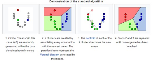
The third novel method is a clustering approach intended to use an advanced method of classifying flowrates with the aim of isolating dry weather flows from other groupings of daily total flows. Taken from machine learning techniques, K-means clustering seeks to sort a series of observations into a number (k) of groups called clusters, thereby revealing underlying patterns. The number of clusters is specified by the user and an algorithm seeks to select centroids such that the distance from that centroid to points within its cluster is minimised. In the case of ADWF, clusters are selected such that similar daily flowrates are grouped together. A real-life analogue might be a four-cluster grouping such as: dry weather, light rain, heavy rain, and extreme weather. Figure 1 demonstrates the idea of K-means clustering.

Figure 1: Diagram of K-means Clustering (Wikipedia, 2020c)

Diurnal profile smoothing

Figure 2: Gaussian Kernel Smoothing (Wikipedia, 2020b)

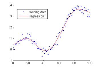
The fourth novel method is an advanced classification method attempting to discern base flowrates from short time-interval data (intervals of minutes or hours). The Diurnal Profile Smoothing method is predicated on identifying higher flow rates indicative of wet weather and separating these from the dry weather flow pattern of an STP. This is possible using large datasets of short time-interval flow rate to overlay plots at weekly time spans. Removing outliers (identified wet weather data) and averaging or smoothing the dry weather weekly flow pattern, produces an estimate of the underlying base flow.

Once the underlying base flow pattern is known, ADWF can be calculated by integration. Figure 2 shows an example of the curves produced by a Gaussian Kernel Regression (the method of smoothing we have chosen).

Kernel density estimation

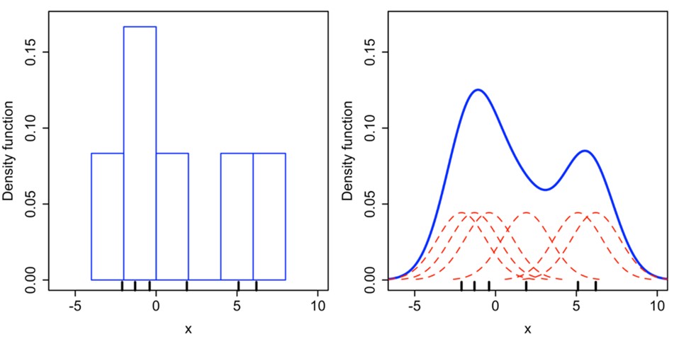
The fifth novel method is a modified histogram/ mode approach that attempts to create a continuous distribution from flow data rather than the discrete formulation of a histogram. The translation to average dry weather flow is the same as for a regular histogram, namely that the most common flowrate is likely to be a good estimate of ADWF.

Kernel density estimation produces a continuous distribution by plotting all the data points (flowrate) onto the X-axis and assigning a distribution function for each point, called a kernel. In the case of Figure 3, a Gaussian distribution has been assigned and centred at each data point (dashed red lines). The final distribution is obtained by summing the values of the individual kernel at continuous x values, resulting in peaks for ranges with many data points and troughs for ranges with few.

Kernel density estimation has two advantages. Firstly, it produces a clearer picture when there are relatively few data points, compared with a histogram. Secondly, it provides weighting to adjacent data points so that a more representative estimate between data points and at extremes is created, which can improve performance with smaller and/or skewed data sets.

Figure 3: Histogram vs Kernel Density Estimation (Wikipedia, 2020a)

Results

Basic statistical methods

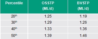
A summary of the results for the Percentile-based methods is given in Table 1.

Table 1: Summary of Percentile-based Estimates

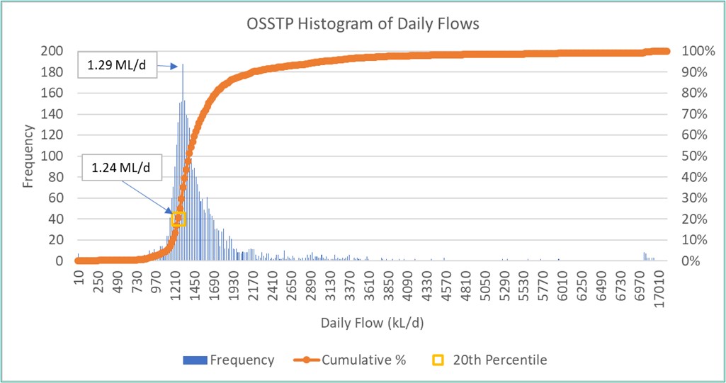
It is useful to compare the percentile results with the mode and traditional histogram for the same datasets. Using the original flow datasets (without editing i.e., including potential outliers) and taking the mode as an estimate for the ADWF, results in a value of 1.29 ML/d and 1.16 ML/d for OSSTP and BVSTP respectively. As an example, the histogram for OSSTP is shown in Figure 4, where the probability plot and 20^th percentile are also plotted, demonstrating similarity between the methods.

Figure 4: OSSTP Daily Flow Histogram

Rainfall-based

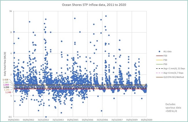
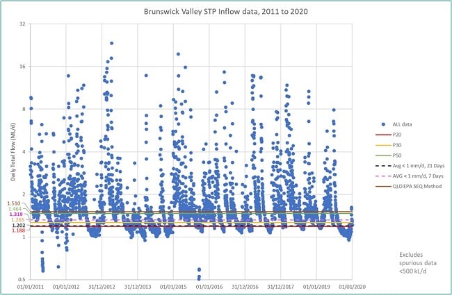
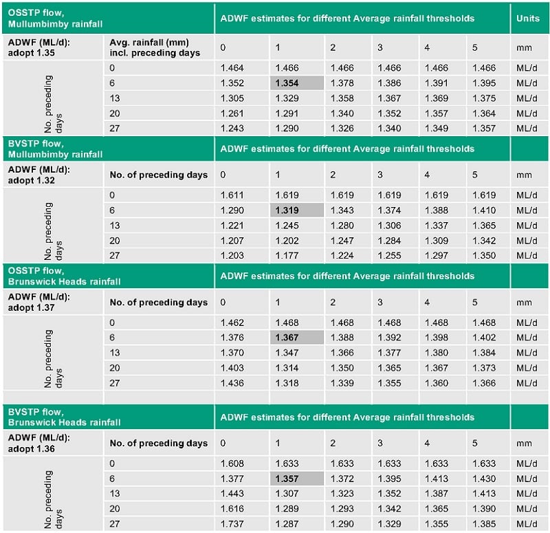
The calculated ADWF was analysed for sensitivity to the number of preceding days considered, and the average rainfall over that period (i.e., a given day and its preceding days). Refer to Table 12 in Supplementary Information for the detailed results. It was concluded that considering at least six preceding days and allowing up to 7 mm cumulative rainfall over that day and its six preceding days, gave a sufficiently strict definition of a dry day. This amounted to an average rainfall of up to 1 mm/day over seven consecutive days. It enabled an estimate of ADWF to within a margin of 10% of the results produced by the strictest parameters tested. The strictest parameters tested were 27 preceding days and 0 mm/d of average rainfall (i.e., 0 mm rainfall on any given day and in aggregate over 28 days). By way of illustration, the ADWF estimated by allowing 1 mm/d average rainfall over one week (i.e., either <7 mm in aggregate over seven consecutive days), or three weeks (i.e., <21 mm in aggregate over 21 days) are both shown in Figure 5 and Figure 6 below for OSSTP and BVSTP, respectively.

Figure 5: Ocean Shores STP Comparison of Existing Methods

Figure 6: Brunswick Valley STP Comparison of Existing Methods

The Rainfall methods can be compared with the Percentile method. The ADWF estimated from the rainfall using the stricter definition of a dry day (<21 mm in aggregate over 21 days) lay between the 20^th and 30^th percentiles, whereas that estimated using (<7 mm in aggregate over 7 days) lay between the 30^th and 50^th percentiles (see Figure 5 and Figure 6). The ADWF estimated from rainfall using a method applied in a recent Queensland STP environmental license (QLD EPA, 2020) was higher than the 50^th percentile (i.e., significantly higher than that from the stricter rainfall definitions applied here - see above).

Novel estimation methods

Antecedent Precipitation Index (API) method

The results for the API method are summarised in Table 2. Like the rainfall method results (see above), the ADWF estimates lay between the 20^th and 30^th percentiles (Table 1).

Table 2: ADWF estimates by API method

Ratio of short term and long-term moving averages

Taking the ADWF as either the mean or median of flows classified as dry by the ratio of moving averages method yields the results in Table 3.

Table 3: ADWF Estimates by Ratio of Moving Averages method

Looking at the ADWF calculated from the mean flows on dry days, the arithmetic moving average and EWMA methods vary by less than 0.05 ML/d without the step-change limit, and by less than 0.03 ML/d with the step-change limit. With the parameters chosen, the two methods for calculating moving averages are almost indistinguishable in terms of ADWF estimated.

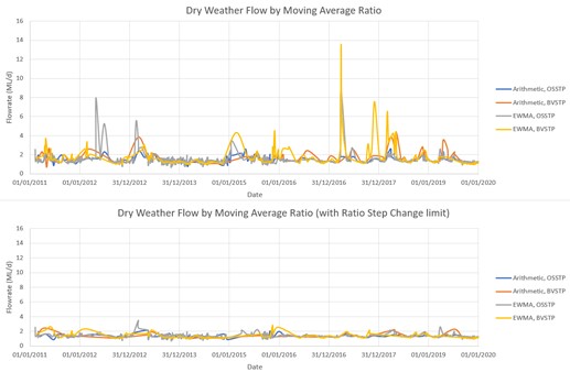
However, the step-change limit had a significant effect on the ADWF estimate (from the mean flows on dry days), particularly for BVSTP where it lowered the estimate from 1.39 to 1.23 ML/d (i.e., by a margin of 11%). Figure 7 illustrates the residual effects of wet weather impacts on flow rates for dry days, as defined by the moving average methods for the two STPs. Anecdotally, BVSTP is more prone to high wet weather flows than OSSTP.

Noting the impact of the step-change limit on the estimated ADWF using the moving average methods, as an alternative, we found that the effect of peak weather events could be reduced in the calculation by replacing mean flow on dry days with the median flow (on dry days). A comparison can be made from the results in Table 3. The median consistently predicts a lower ADWF than the mean and gives very little change in the result when altering or completely removing the step-change limit. With or without the step-change limit, the ADWF estimate changed by 0.02 ML/d or less (a margin of <2%).

Figure 7: Dry Weather Flow as defined by Ratio of Moving Averages (BVSTP and OSSTP)

K-means clustering

Figure 8: K-means Clustering results for OSSTP and BVSTP

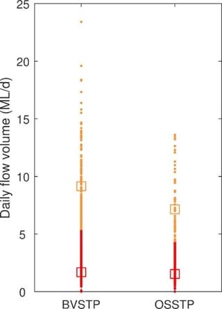
Data was tested from two to ten clusters (k=2 to k = 10) and the number of clusters that best grouped the data was used (as measured by the Silhouette coefficient). The Silhouette Coefficient (minimum is -1, maximum is +1) is dimensionless. It is used as a measure of clustering for a dataset with a larger value (closer to +1) indicating better clustering. The Silhouette Coefficient for the two datasets in Figure 8 ranged from 0.6 to 1.

The results of K-means clustering on OSSTP and BVSTP are displayed below in Figure 8 for k = 2, as this gave the highest Silhouette Coefficient. The final Silhouette Coefficients were 0.97 and 0.95 for OSSTP and BVSTP, respectively.

ADWF was estimated by the centroid of the lowest cluster (red square in Figure 8, and the results are shown below in Table 4.

Compared with results for other methods (see above), the K-means Cluster estimates of ADWF (Table 4) were relatively high and likely to be over-predicting ADWF. This is due to a relatively uniform distribution of flowrates in the datasets (see Figue 8). The underlying cause is the I/I pattern, influenced largely by climate, location and the nature of sewer catchments served by the STPs. It was noted that this method performed well when tested on a STP in North Queensland where the flow pattern is more multimodal. Multimodal flow patterns would be characterised by two or more distinctly different sets (or clusters) of flowrates, for example, a distinct wet season vs. dry season, which tends to be characteristic of North Queensland.

Table 4: K-means Clustering Results

Diurnal profile smoothing

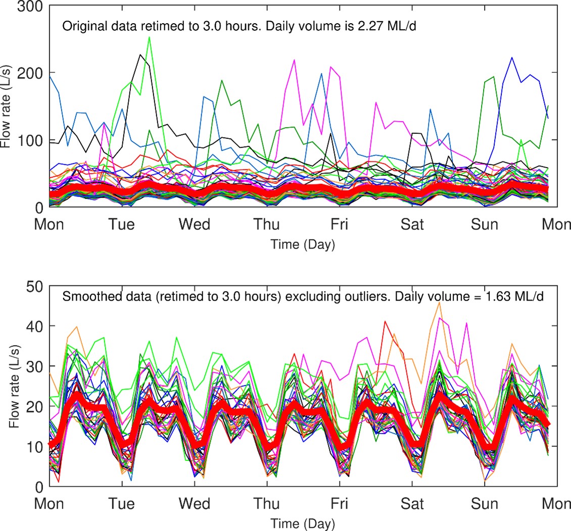
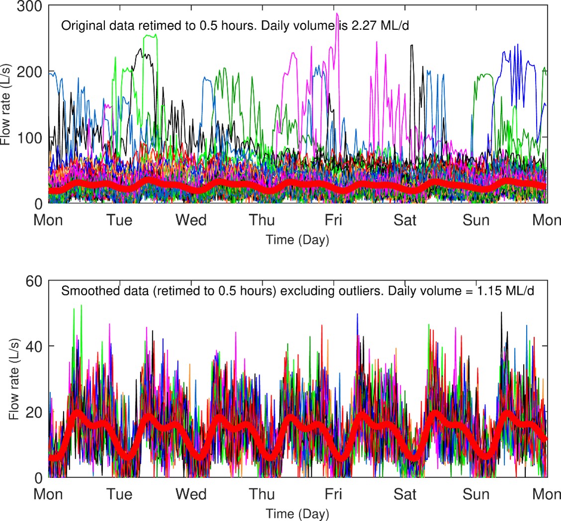
Plots of 3-hour and 0.5-hour aggregations of diurnal flow rates using the Diurnal Smoothing Method are shown below in Figure 9 and Figure 10 for BVSTP data. This method was not tested for OSSTP data, due to study constraints. The ADWF results for both calculations are presented in Table 5.

Table 5: Diurnal Profile Smoothing Results

Table 5 shows that the results are sensitive to the time interval chosen. To obtain an accurate estimate of ADWF, namely that aligned with existing methods, the time interval had to be decreased to 0.5 hours. The ADWF estimate was 1.15 ML/d, which aligns closely with that from other methods (e.g., the Percentile or Rainfall-based methods – see Figure 6). The inclusion of outliers at the same time interval gave a result of 2.27 ML/d (Table 5), demonstrating the importance of removing outlier weekly profiles when using this method.

Figure 9: BVSTP Diurnal Smoothing (3 Hour data aggregation)

Figure 10: BVSTP Diurnal Smoothing (0.5 Hour data aggregation)

Kernel density estimation

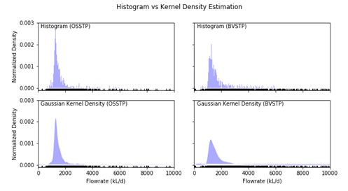
Kernel density estimation was performed on both OSSTP and BVSTP using all daily flow data, including potentially spurious data. The distributions are shown below in Figure 11. It can be seen in the figure that the histogram is jagged while the Kernel density distribution is smooth. For BVSTP, the mode is at 1.29 ML/d while the Kernel density estimate is 1.22 ML/d, highlighting the advantage of this method.

Figure 11: Kernel Density Estimation Results

Using the peak of the continuous curves (Gaussian Kernel Density distributions) as the estimate for ADWF for each plant produces the results in Table 6. The results for both STPs align well with the previous high performing methods (e.g., ratio of moving averages), as well as the existing ‘Strictest’ methods (e.g., Percentile or Rainfall-based).

Table 6: Kernel Density Estimation Results

Discussion

A multi-criteria assessment (MCA) approach was used to review and compare all the ADWF estimation methods (existing and novel) developed and/or tested in this study.

Estimation classifications

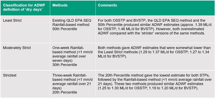
Rating estimates of ADWF as ‘good’ or ‘bad’ is to some extent subjective, given that the true ADWF value is uncertain and the estimation methods differ in complexity, which is a user judgement. To meaningfully discuss the results of different estimates, we applied a classification system based on ‘strictness’. Based on preliminary results from existing methods commonly used in industry and the literature (i.e., Flow percentile and Rainfall-based methods), we adopted three nominal classifications that hinge on the definition of ‘dry days’: ‘Least Strict’, ‘Moderately Strict’, and ‘Strictest’, as summarised in Table 7 below.

Table 7: Classification of existing methods used for assessment in this study

Multi-Criteria Assessment (MCA)

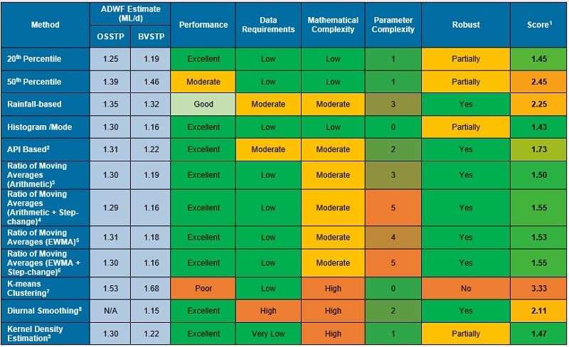
To assess the ability for each method to accurately estimate ADWF, a ‘true value ADWF’ needed to be established for each STP. The ‘Strictest’ method estimates were approximately 1.30 ML/d for OSSTP and 1.20 ML/d for BVSTP. Whilst most of the novel methods gave results that agreed closely with this estimate for OSSTP, a number produced lower estimates for BVSTP.

The adopted ‘true’ ADWF value was chosen based on the average of the high performing methods (i.e., methods giving estimates closest to those using the ‘Strictest’ methods classified in Table 7 and in closest agreement with each other), namely: Histogram/ Mode, API, Ratio of Moving Averages, Diurnal Smoothing, and Kernel Density Estimation.

The adopted ‘true’ ADWF values were 1.30 ML/d for OSSTP and 1.18 ML/d for BVSTP.

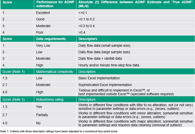
Methods were then scored (Table 8) based on their ADWF estimates for both STPs, using the sum of the difference between the method estimates and the adopted ‘True ADWF’ values.

Since estimation performance is similar among many of the high-performing methods, additional criteria were considered in the MCA. These criteria were data requirements, mathematical complexity, parameter complexity, and robustness (e.g., sensitivity to choice of parameters; sensitivity to data errors). The scoring criteria for these are also listed below in Table 8. For all criteria, a low score value is better.

Table 8: MCA Scores for Criteria

The scores against all criteria for characteristics were summed and weightings applied to determine the overall score for a given method. The weightings are given in Table 9.

Table 9: MCA Weightings

The results of the MCA are presented in Table 10.

Table 10: Summary of Methods & MCA Analysis

[1] A lower score is better

[2] Decay Constant = 0.9, API Limit = 10, Median.

[3] Long term days = 28, Short term days = 7, Upper Bound = 1.025, Median.

[4] Long term days = 28, Short term days = 7, Upper Bound = 1.025, Step-change limit = 0.025, Median.

[5] Long term days = 28, Short term days = 7, Upper Bound = 1.025, Decay constant = 0.9, Median.

[6] Long term days = 28, Short term days = 7, Upper Bound = 1.025, Decay constant = 0.9, Step-change limit = 0.025, Median.

[7] K = 2

[8] Bandwidth = 2 hours, Outlier Factor = 5 relative to Median

[9] Bandwidth = Silverman’s rule of thumb

Based on the data analysis and MCA undertaken for this study, the following observations are made regarding the various methods for ADWF estimation:

• The Percentile method can estimate ADWF very well, provided the appropriate percentile is chosen and the data has been filtered for errors and outliers. However, the appropriate percentile might vary depending on location and a degree of user input is required for data checking since the calculated percentile is somewhat sensitive to potential data errors (e.g., zeroes and outliers).
• The Histogram/ Mode method can estimate ADWF very well and is easy to perform. This method might require some degree of interpretation depending on location (if non-dry weather flows are very common). The Histogram is also useful in that it gives the user an opportunity to visualise the whole dataset, including outliers and zeroes.
• Rainfall-based methods can estimate ADWF very well with reasonably large datasets, provided strict rainfall thresholds are set. However, these methods require both daily flow data and daily rainfall data. The definition of appropriate rainfall thresholds might vary, depending on location, and proximity of the plant to a weather station with reliable rainfall records might be a constraint.
• The Ratio of Moving Averages method can estimate ADWF very well and does not require rainfall data. However, it requires a degree of user input for data manipulation and calibration around selection of upper and lower ratio bounds. Further notes for this method are:
• Applying a step-change limit significantly improves the performance of the ratio of moving averages method when using mean (average) flow to calculate ADWF; whereas
• Using the median flow instead of mean flow to calculate ADWF improves robustness of the ratio of moving averages method, largely eliminates the need for a step-change limit and reduces sensitivity to outlier data.
• K-means clustering can be effective for multi-modal flowrates. However, this method is not useful if flowrates are relatively uniformly distributed. This makes the method potentially sensitive to the location and nature of the sewer catchments.
• Diurnal Profile Smoothing can produce excellent estimates of ADWF, but it is much more mathematically complex and ‘data heavy’ since it requires short time interval flow data (hours or minutes) and outlier algorithms.
• Kernel Density Estimation can improve upon the Histogram/ Mode approaches where the number of data points is limited, or data is skewed. In most other respects, it does not offer significant advantages over simpler methods, given the disadvantage that it is mathematically complex.
• Several of the methods tested produce similar estimates of ADWF that can be considered reliable. Selection of the most appropriate method will likely depend on a balance of data requirements, mathematical simplicity (or complexity), and robustness (i.e., the extent to which user input/ interpretation required).

Conclusion

A review of existing industry ‘best practice’ methods for estimating ADWF at sewage treatment plants revealed that the current methods fall into three groups: Rainfall-based, EP-based, and Basic Statistical. Several potential Novel methods were also identified as a fourth group. Of those groups, Rainfall-based and Basic Statistical were the more common methods currently used. EP-based methods were not compared in this study, as they were considered to move the uncertainty from flow to population data, rather than attempting to directly calculate ADWF.

Based on this study, on balance of simplicity and performance against more complex methods, we recommend either or both of the following methods for routine estimation of ADWF at sewage treatment plants:

• Histogram/ Mode method - Plot histogram and/or calculate mode for datasets that are reasonably large (indicatively at least one year of daily STP total flow readings). Some user discretionary checking of data (at least from visual checks of histogram plots of raw data) is recommended to identify false zeroes and potential outliers, from which data filtering or outlier tests might be required.
• Percentile method: Adopt 20^th percentile as a default, but with user discretion to check data (at least from visual checks of histogram plots of raw data, or using outlier tests), followed by minor sensitivity checks (e.g., test 20^th, 30^th and 50^th percentiles).

For larger and more complex assignments (e.g., design projects, planning studies), it is recommended that one or more of the alternative high-performing methods described in this paper (e.g., Ratio of moving averages; Kernel Density Estimation) be employed for ADWF checks. Relatively large datasets (at least one year of daily flow totals) should be used and the results compared against the estimates from simpler methods (e.g., Histogram/ Mode and/ or Percentile methods).

Acknowledgements

We gratefully acknowledge the assistance of Anjila Finan (Byron Shire Council) with flow data collation and transmittal.

About the authors

Dr David de Haas | Dr David de Haas is a Senior Technical Director at GHD Pty Ltd with specialist skills in wastewater treatment systems. He has thirty-five years’ experience in municipal water and wastewater treatment, covering research and development, planning, process design and operation. He has worked in wastewater-related consultancy in Australia for more than twenty years.

Stuart Ng | Stuart Ng is a Process Engineer at GHD Pty Ltd with skills in modelling and optimisation of wastewater treatment systems. He has 2 years' experience in process engineering, including hands-on operation and optimisation at a brewery waste treatment plant.

Nick Dahl | Nick Dahl is a Civil Engineer at GHD Pty Ltd with five years’ experience, specialising in modelling water, wastewater and sewer systems, including the effects of rainfall. His work includes the use of InfoWorks ICM (integrated with ArcGIS), supplemented with the development of a range of analytics tools using MATLAB.

Dean Baulch | Dean Baulch is a Principal Engineer (Systems Planning, Utilities) at Byron Shire Council, a role he has filled for twelve years. He has thirty years of experience in the water industry, including planning, design, management and operation of urban water and wastewater systems.

Supplementary information

Table 11: Summary of Existing ADWF Estimation Methods

[10] Determine unit flow (L/EP) at ADWF for detached residential development based on internal water consumption and/or bulk metering of a residential catchment, and occupancy ratio. Determine total EP and total ADWF for detached residential development or land use. Determine unit flow (L/EP) at ADWF for all other (excluding detached residential) land use categories and/ or development/ customer categories. For all categories determine total EP and ADWF. Alternatively, where possible, determine total ADWF from treatment plant and catchment metering. Calibrate ADWF calculated from treatment plant or catchment metering against the calculated ADWF based on L/EP based land use categories. (Queensland Water Supply Regulator, Water Supply and Sewerage Services, Department of Energy and Water Supply, 2014).

Table 12: Summary of ADWF Estimates Using Rainfall Method for Two STPs

References

Ali, S., Ghosh, N. C., & Singh, R. (2010, Mar 24). Rainfall-runoff simulation using normalized antecedent precipitation index. Hydrological Science Journal - Journal Des Sciences Hydrologiques, 55(2), 226-274.

City of Winnipeg. (2020). Wastewater Flow Estimation and Servicing Guidelines. Retrieved from Winnipeg Water and Waste Department, Winnipeg Manitoba: https://winnipeg.ca/waterandwaste/dept/wastewaterFlow.stm

Elias-Maxil, J. A., Hoek, J. P., Hofman, J., & Rietveld, L. (2014). A bottom-up approach to estimate dry weather flow in minor sewer networks. Water Science & Technology. 69.5, pp. 1059-1066. IWA Publishing.

GHD. (2017). Rainfall Analysis for Mullumbimby and Brunswick Heads WWTPs.

Kohler, M., & Linsley, R. (1951). Predicting The Runoff From Storm Rainfall. Washington: National Oceanic & Atmospheric Administration U.S. Dept. of Commerce.

Murray, N., Gabbett, T., & Townshend, A. (2017). Calculating acute:chronic workload ratios using exponentially weighted moving averages provides a more sensitive indicator of injury likelihood than rolling averages. British Journal of Sports Medicine, 51, 749-754.

NSWEPA. (2020). Environment Protection License 1802 for Kincumber Sewage Treatment System, Central Coast Council. Retrieved from NSW Environmental Protection Agency, Sydney: https://apps.epa.nsw.gov.au/prpoeoapp/

QLDEPA. (2019). Environmental Authority EPPR00887713 for Cairns Regional Council. Retrieved from Queensland Department of Environment and Science: https://apps.des.qld.gov.au/env-authorities/map/

QLDEPA. (2020). Environmental Authority EPPR00521513 for Queensland Urban Utilities. Retrieved from Queensland Department of Environment and Science: https://apps.des.qld.gov.au/env-authorities/map/

Queensland Water Supply Regulator, Water Supply and Sewerage Services, Department of Energy and Water Supply. (2014). Planning Guidelines for Water Supply and Sewerage. Retrieved from Queensland Government, Brisbane: https://www.dews.qld.gov.au/__data/assets/pdf_file/0016/80053/water-sewerage-planning-guidelines.pdf

UK Gov Environment Agency. (2018). Guidance Calculating dry weather flow (DWF) at waste water treatment works. Retrieved from United Kingdom Government, London: https://www.gov.uk/government/publications/calculating-dry-weather-flow-dwf-at-waste-water-treatment-works/calculating-dry-weather-flow-dwf-at-waste-water-treatment-works

USEPA. (2014). Guide for Estimating Infiltration and Inflow. Retrieved from United States Environmental Protection Agency, Washington DC: https://www3.epa.gov/region1/sso/pdfs/Guide4EstimatingInfiltrationInflow.pdf

Wikipedia. (2020a, July 21). Kernel density estimation. Retrieved from Wikipedia: https://en.wikipedia.org/wiki/Kernel_density_estimation

Wikipedia. (2020b, Jul 21). Kernel smoother. Retrieved from Wikipedia: https://en.wikipedia.org/wiki/File:Gaussian_Kernel_Regression.png

Wikipedia. (2020c, July 21). K-means clustering. Retrieved from Wikipedia: https://en.wikipedia.org/wiki/K-means_clustering

WSSA. (2014). Gravity Sewerage Code of Australia WSA Third Edition. Docklands, Victoria: Water Services Association of Australia Limited.